Modeling the COVID-19 Pandemic
Contents
Modeling the COVID-19 Pandemic
Reading
Bregman D.J., A.D. Langmuir, 1990. Farr’s law applied to AIDS projections. JAMA, 263:1522–1525. doi: 10.1001/jama.263.11.1522.
King, A.A., M.D. de Cellès, F.M.G. Magpantay, and P. Rohani, 2015. Avoidable errors in the modelling of outbreaks of emerging pathogens, with special reference to Ebola, Proc. R. Soc. B. 28220150347 http://doi.org/10.1098/rspb.2015.0347.
Murray, C.J.L., and IHME COVID-19 health service utilization forecasting team, 2020. Forecasting COVID-19 impact on hospital bed-days, ICU-days, ventilator-days and deaths by US state in the next 4 months, https://www.medrxiv.org/content/10.1101/2020.03.27.20043752v1.full-text
Jewell, N.P., J.A. Lewnard, and B.L. Jewell, 2020. Predictive Mathematical Models of the COVID-19 Pandemic: Underlying Principles and Value of Projections, JAMA, 323(19):1893-1894. doi:10.1001/jama.2020.6585
Froese, H., 2020. Infectious Disease Modelling: Fit Your Model to Coronavirus Data, Towards Data Science, https://towardsdatascience.com/infectious-disease-modelling-fit-your-model-to-coronavirus-data-2568e672dbc7; https://github.com/henrifroese/infectious_disease_modelling
Smith, D., and L. Moore, 2004. The SIR model for spread of disease, Convergence, https://www.maa.org/press/periodicals/loci/joma/the-sir-model-for-spread-of-disease-introduction
Models of epidemics
This notebook explores two basic approaches to modeling the spread of a communicable disease through a population. There are more complicated approaches than are considered here, but these are common, and the predictions of COVID-19 infections, ICU beds, and deaths are often based on variations of these models.
SIR models
Mathematical models of epidemics date back to the early 1900s.
One of the simplest models of epidemics is the SIR model, which partitions the population into three disjoint groups: Susceptible, Infected, and Recovered (or Removed).
The SIR model treats the population as fixed: no births, immigration, emigration, or deaths from other causes. It ignores the possibility of carriers, population heterogeneity, or geographic heterogeneity. It treats everyone as equivalent and assumes the population “mixes” perfectly.
Here are the state variables of the SIR model:
\(N\): initial population size
\(S(t)\): number of susceptible individuals in the population at time \(t\)
\(I(t)\): number of infected individuals in the population at time \(t\)
\(R(t)\): number “removed” from risk (dead or recovered) in the population at time \(t\)
Assumptions:
Everyone is either susceptible, infected, or removed (recovered or dead). (There are more complex models with more “compartments.”)
There are no births, immigration, emigration, or deaths from other causes.
If a susceptible person is infected, that person eventually dies or recovers.
While a person is infected, the person is infectious.
There is no incubation period between being infected and being infectious.
If an infected person gets “close enough” to a susceptible person, the susceptible person becomes infected.
Every unit of time, every infected person exposes \(\beta\) people.
Every susceptible person exposed to an infected person becomes infected.
Every infected person exposes a disjoint group of people.
Every unit of time, a fraction \(\gamma\) of infected people recover or die.
People who recover or die are not infectious.
People who recover or die never become susceptible again.
Then \(S + I + R = N\) is constant, the initial population size.
The basic reproductive number is \(R_0 = \beta/\gamma\). Initially, when essentially the entire population is susceptible (the proportion who are infected or recovered is small compared to \(N\)), this is the number of people each infected person infects before recovering or dying. (Note that \(R_0\) has no connection to \(R\): the notation is unfortunate.)
Define \(s(t) \equiv S(t)/N\), \(i(t) \equiv I(t)/N\), and \(r(t) \equiv R(t)/N\). Then \(s+i+r = 1\) for all \(t\). There is an epidemic if \(s(0)\beta/\gamma > 1\): the rate at which susceptible people are getting infected is greater than the rate at which infected people are recoving.
The parameters of the model are:
\(\beta\), the number of exposed people per unit of time per infected persion
\(\gamma\), the fraction of infected people who are removed (recover or die) per unit time
The state of the population evolves according to three coupled differential equations:
\(dS/dt = -\beta I S/N\)
\(dI/dt = \beta I S/N - \gamma I\) (equivalently, \(di/dt = \beta is - \gamma i\))
\(dR/dt = \gamma I\)
Another interesting variable is the cumulative number of infections, \(C\).
\(dC/dt = \beta I S/N\); \(C(0) = I(0)\).
The SIR model has some built-in features that might not match reality. First, note that the derivative of \(R\) is always non-negative and proportional to \(I\). Since \(R \le N\) and \(N\) is finite, \(I\) must eventually be zero; that is, the SIR implies that eventually the entire population will be disease-free. Once \(I=0\), it can never grow again, since the derivative of \(I\) is proportional to \(I\). (If nobody is infected, nobody can infect anyone.) Epidemics that follow the SIR model are necessarily self-limiting.
That isn’t the case if immunity wears off over time (or if the population is not isolated). In that case, we might we parametrize the transition from recovered to susceptible by assuming that a fraction \(\delta\) of \(R\) return to \(S\) in each time period. (There are other ways we could do this, for instance, having a variable “lag” between recovery and becoming susceptible again.) That yields:
\(dS/dt = -\beta I S/N + \delta R\)
\(dI/dt = \beta I S/N - \gamma I\) (equivalently, \(di/dt = \beta is - \gamma i\))
\(dR/dt = \gamma I - \delta R\)
In this model, \(I\) does not necessarily go to zero eventually.
Other generalizations include separate “compartments” for dead versus recovered), needing an ICU bed, etc., as well as time-varying values of \(\beta\) to account for lockdowns or other policy interventions, heterogeneity in the population, and more.
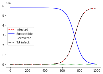
Let’s run this model (in discrete time) for a population of \(N=1,000,000\) people of whom 0.05% are initially infected. We will take the time interval to be 1 day, the period of infectiousness to be \(1/\gamma = 14\) days, and \(R_0 = 2 = \beta/\gamma\), so \(\beta = 2 \gamma = 1/7\). We will start with \(\delta=0\) (no re-infections).
# boilerplate
import numpy as np
import scipy as sp
from scipy.integrate import odeint
import matplotlib.pyplot as plt
import matplotlib.dates as mdates

from ipywidgets import interact, interactive, fixed, interact_manual
import ipywidgets as widgets
from IPython.display import clear_output, display, HTML
def sir_model(N, i_0, beta=1, gamma=1, delta=0, steps=365):
    '''
    Run SIR model as coupled finite-difference equations.

    Assumes that initially a fraction i_0 of the population of N people is infected and
    everyone else is susceptible (none has died or recovered).

    Parameters
    -----------
    N     : int
        population size
    i_0   : double in (0, 1)
        initial fraction of population infected
    beta  : double in [0, infty)
        number of encounters each infected person has per time step
    gamma : double in (0, 1)
        fraction of infecteds who recover or die per time step
    delta : double in (0, 1)
        fraction of recovereds who become susceptible per time step
    steps : int
        number of steps in time to run the model

    Returns
    --------
    S, I, R, C
    S     : list
        time history of susceptibles
    I     : list
        time history of infecteds
    R     : list
        time history of recovered/dead
    C     : list
        cumulative number of infections over time
    '''
    assert i_0 > 0, 'initial rate of infection is zero'
    assert i_0 <= 1, 'infection rate greater than 1'
    assert beta >= 0, 'beta must be nonnegative'
    assert gamma > 0, 'gamma must be positive'
    assert gamma < 1, 'gamma must be less than 1'
    assert delta >= 0, 'delta must be nonnegative'
    assert delta < 1, 'delta must be less than 1'
    S = np.zeros(steps)
    I = np.zeros(steps)
    R = np.zeros(steps)
    C = np.zeros(steps)
    I[0] = int(N*i_0)
    C[0] = I[0]
    S[0] = N-I[0]
    for i in range(steps-1):
        new_i = beta*I[i]*S[i]/N
        S[i+1] = max(0, S[i] - new_i + delta*R[i])
        I[i+1] = max(0, I[i] + new_i - gamma*I[i])
        R[i+1] = max(0, R[i] + gamma*I[i] - delta*R[i])
        C[i+1] = C[i] + new_i
    return S, I, R, C
def plot_sir(N, i_0, beta=2/14, gamma=1/14, delta=0, steps=365, verbose=False):
    '''
    Plot the time history of an SIR model.

    Parameters
    -----------
    N     : int
        population size
    i_0   : double in (0, 1)
        infection rate at time 0
    beta  :  double in [0, infty)
        number of encounters each infected person has per time step
    gamma : double in (0, 1)
        fraction of infecteds who recover or die per time step
    delta : double in (0, 1)
        fraction of recovereds who become susceptible per time step
    steps : int
        number of time steps to run the model
    verbose : Boolean
        if True, return the model predictions

    Returns (if verbose == True)
    --------
    S : list
        susceptibles as a function of time
    I : list
        infecteds as a function of time
    R : list
        recovereds as a function of time
    C : list
        cumulative incidence as a function of time
    '''
    S, I, R, C = sir_model(N, i_0, beta=beta, gamma=gamma, delta=delta, steps=steps)
    times = list(range(steps))
    fig, ax = plt.subplots(nrows=1, ncols=1)
    ax.plot(times, I, linestyle='--', color='r', label='Infected')
    ax.plot(times, S, linestyle='-', color='b', label='Susceptible')
    ax.plot(times, R, linestyle=':', color='g', label='Recovered')
    ax.plot(times, C, linestyle='-.', color='k', label='Tot infect.')
    ax.legend(loc='best')
    plt.show()
    if verbose:
        return S, I, R, C
i_0 = 0.0005
N = int(10**6)
steps = 365

plot_sir(N, i_0)
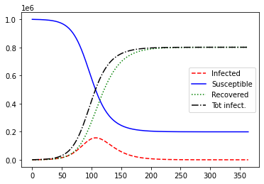
For these parameters, the number of infections is shaped like a bell curve and the cumulative number of infections is shaped like a CDF: it is “sigmoidal” (vaguely “S”-shaped). You might imagine fitting a scaled CDF to the curve. Essentially, the IHME model fits a scaled Gaussian CDF to the total number of infections. (More on this below.)
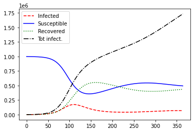
What if immunity wears off over time? Let’s try a positive value of \(\delta\):
plot_sir(N, i_0, delta=0.01)
interact(plot_sir, N=fixed(N),
                   i_0 = widgets.FloatSlider(min=0, max=1, value=i_0),
                   beta=widgets.FloatSlider(value=2/14, min=0.01, max=100),
                   gamma=widgets.FloatSlider(value=1/14, min=0, max=1, step=0.01),
                   delta=widgets.FloatSlider(value=0, min=0, max=1, step=0.01),
                   steps=fixed(steps),
                   verbose=fixed(False))
<function __main__.plot_sir(N, i_0, beta=0.14285714285714285, gamma=0.07142857142857142, delta=0, steps=365, verbose=False)>
Fitting the SIR model to data
Now we will use least squares to fit the SIR model to a time history of infection data collected by researchers at Johns Hopkins University. See https://github.com/CSSEGISandData
This exercise is for illustration. There are many reasons to be wary of this modeling:
There are serious issues with the data quality: these are cases that were reported according to the rules and circumstances of where they were detected. For mortality (rather than incidence), excess mortality might give a more accurate measure.
The model is a cartoon, not “physics” of epidemics, and it omits many factors that plausibly matter. It is not clear what estimates of the parameters mean when the model is wrong.
Absent a trustworthy generative model for the data, it is not clear how to assess or interpret the uncertainty of the estimates.
If the estimated model is to be used for prediction, there is no obvious way to assign meaningful uncertainties to the predictions.
The optimization problem to fit the parameters has no statistical content or motivation. It is not clear that it yields an estimate that is “good” in a useful sense.
The objective function is not convex in the model parameters, and the optimization algorithm is not guaranteed to solve the optimization problem.
The data record total “confirmed” cases as a function of time, deaths, and recoveries: \(C(t)\)
from scipy.optimize import curve_fit  # nonlinear least squares

def f(x, beta, gamma):
    '''
    Model cumulative infections

    This is just a wrapper for a call to sir_model, to generate a set of
    predictions of the cumulative incidence for curve fitting
    '''
    return sir_model(N, i_0, beta, gamma, delta=0, steps=len(x))[3]  # C
# test f
N = int(10**6)
i_0 = 0.0005
x = range(25)
y = f(x, 1/7, 1/14 )
y
array([ 500.        ,  571.39285714,  647.87464122,  729.80689646,
        817.5766761 ,  911.59831599, 1012.31532767, 1120.20241833,
       1235.76764552, 1359.55471484, 1492.14542917, 1634.1622985 ,
       1786.27131969, 1949.18493587, 2123.66518564, 2310.5270524 ,
       2510.64202461, 2724.94187786, 2954.42268994, 3200.14910031,
       3463.25882519, 3744.96743963, 4046.57343789, 4369.46358264,
       4715.11855381])
# test curve_fit
popt, pvoc = curve_fit(f, x, y, p0=[1, 0.5], bounds = (0, [np.inf, 1]))
popt
array([0.14285714, 0.07142857])
# try some real data from the JHU site
import pandas as pd
# data for countries. THIS IS A "LIVE" DATASET THAT IS UPDATED FREQUENTLY
url = "https://raw.githubusercontent.com/CSSEGISandData/COVID-19/master/csse_covid_19_data/csse_covid_19_time_series/time_series_covid19_confirmed_global.csv"
df = pd.read_csv(url, sep=",")
df.head()
| Province/State | Country/Region | Lat | Long | 1/22/20 | 1/23/20 | 1/24/20 | 1/25/20 | 1/26/20 | 1/27/20 | ... | 3/4/22 | 3/5/22 | 3/6/22 | 3/7/22 | 3/8/22 | 3/9/22 | 3/10/22 | 3/11/22 | 3/12/22 | 3/13/22 | |
|---|---|---|---|---|---|---|---|---|---|---|---|---|---|---|---|---|---|---|---|---|---|
| 0 | NaN | Afghanistan | 33.93911 | 67.709953 | 0 | 0 | 0 | 0 | 0 | 0 | ... | 174214 | 174331 | 174582 | 175000 | 175353 | 175525 | 175893 | 175974 | 176039 | 176201 |
| 1 | NaN | Albania | 41.15330 | 20.168300 | 0 | 0 | 0 | 0 | 0 | 0 | ... | 272030 | 272030 | 272210 | 272250 | 272337 | 272412 | 272479 | 272552 | 272621 | 272663 |
| 2 | NaN | Algeria | 28.03390 | 1.659600 | 0 | 0 | 0 | 0 | 0 | 0 | ... | 265186 | 265227 | 265265 | 265297 | 265323 | 265346 | 265366 | 265391 | 265410 | 265432 |
| 3 | NaN | Andorra | 42.50630 | 1.521800 | 0 | 0 | 0 | 0 | 0 | 0 | ... | 38434 | 38434 | 38434 | 38620 | 38710 | 38794 | 38794 | 38794 | 38794 | 38794 |
| 4 | NaN | Angola | -11.20270 | 17.873900 | 0 | 0 | 0 | 0 | 0 | 0 | ... | 98796 | 98796 | 98806 | 98806 | 98829 | 98855 | 98855 | 98855 | 98909 | 98927 |
5 rows × 786 columns
# data for Denmark
DK = df.loc[(df["Country/Region"] == "Denmark") & df["Province/State"].isna()]  # Denmark
DK = DK.drop(['Province/State','Country/Region','Lat','Long'], axis=1).T        # remove fields we don't need
y = DK.to_numpy()   # turn series into a vector
y = y[np.nonzero(y)] # remove the data before the first detected case
x = range(len(y))    # for model-fitting and plotting
print(len(y),y)
746 [      1       1       3       4       4       6      10      10      23
      23      35      90     262     442     615     801     827     864
     914     977    1057    1151    1255    1326    1395    1450    1591
    1724    1877    2046    2201    2395    2577    2860    3107    3386
    3757    4077    4369    4681    5071    5402    5635    5819    5996
    6174    6318    6511    6681    6879    7073    7242    7384    7515
    7695    7912    8073    8210    8445    8575    8698    8851    9008
    9158    9311    9407    9523    9670    9821    9938   10083   10218
   10319   10429   10513   10591   10667   10713   10791   10858   10927
   10968   11044   11117   11182   11230   11289   11360   11387   11428
   11480   11512   11593   11633   11669   11699   11734   11771   11811
   11875   11924   11948   11962   12001   12016   12035   12099   12139
   12193   12217   12250   12294   12344   12391   12391   12391   12527
   12561   12615   12636   12675   12675   12675   12751   12768   12794
   12815   12832   12832   12832   12878   12888   12900   12916   12946
   12946   12946   13037   13061   13092   13124   13173   13173   13173
   13262   13302   13350   13390   13438   13438   13438   13547   13577
   13634   13725   13789   13789   13789   13996   14073   14185   14306
   14442   14442   14442   14815   14959   15070   15214   15379   15483
   15617   15740   15855   15940   16056   16127   16239   16317   16397
   16480   16537   16627   16700   16779   16891   16985   17084   17195
   17374   17547   17736   17883   18113   18356   18607   18924   19216
   19557   19890   20237   20571   20571   21393   21847   22436   22905
   23323   23799   24357   24916   25594   26213   26637   27072   27464
   27998   28396   28932   29302   29680   30057   30379   30710   31156
   31638   32082   32422   32811   33101   33593   34023   34441   34941
   35392   35844   36373   37003   37763   38622   39411   40356   41412
   42157   43174   44034   45225   46351   47299   48241   49594   50530
   51753   53180   54230   55121   55892   56958   57952   58963   60000
   61078   62136   63331   64551   65808   67105   68362   69635   70485
   71654   73021   74204   75395   76718   78354   79352   80481   81949
   83535   85140   86743   88858   90603   92649   94799   97357  100489
  103564  107116  109758  113095  116087  119779  123813  128321  131606
  134434  137632  140175  143472  146341  149333  151167  153347  155826
  158447  161230  163479  165930  167541  168711  170787  172779  174995
  176837  178497  180240  181486  182725  183801  185159  185159  187320
  188199  189088  189895  190619  191505  192265  193038  193917  194671
  195296  195948  196540  197208  197664  198095  198472  198960  199357
  199782  200335  200773  201186  201621  202051  202417  202887  203365
  203793  204067  204362  204799  205183  205597  206065  206617  207081
  207577  208027  208556  209079  209682  210212  210732  211195  211692
  212224  212798  213318  213932  214326  214839  215264  215791  217798
  218660  219305  219918  220459  221071  221842  222629  223415  224258
  224848  225505  226777  227031  225030  225844  226633  227049  228013
  228692  229902  230603  231265  231973  232718  233318  233797  234317
  234931  235648  236346  237101  237792  238306  238869  239532  240330
  241007  241731  242633  243374  244065  244868  245761  246463  247010
  247622  248326  248950  249785  250554  250554  252045  252912  253673
  254482  254482  256482  257505  258182  259056  259988  260913  262159
  263514  264465  265539  266503  267339  268255  269343  270557  271908
  272659  273494  274413  275207  276280  277399  278396  279434  280383
  281227  282135  283089  284117  285044  285636  286489  286948  287325
  288229  288704  289122  289559  289874  290111  290333  290686  291017
  291220  291463  291652  291801  291956  292179  292352  292574  292769
  292943  293094  293337  293677  294152  294478  294925  295317  295654
  296196  296885  297543  298094  298614  299223  300071  301126  302328
  303469  304429  305459  306100  306944  307764  308615  309420  310127
  310876  311520  312292  312851  314135  314983  316068  316807  317700
  318485  319295  320222  321154  322019  322965  323786  324721  325725
  326887  327972  329010  329927  330777  331736  332622  333815  334799
  335722  336746  337466  338240  339580  340567  341549  342474  343351
  344088  344850  345693  346518  347212  347909  348347  348979  349440
  349891  350405  350996  351553  351939  352373  352636  353061  353431
  353744  354068  354393  354645  354913  355257  355603  355944  356326
  356684  357037  357370  357827  358369  358796  359237  359663  360031
  360411  360888  361461  362068  362738  363356  363900  364464  365051
  365840  366607  367307  368060  368651  369403  370159  371286  372533
  373803  375065  376414  377825  379078  380949  382796  384580  386251
  387783  389240  391221  393199  395797  398048  400145  402561  404855
  407417  410434  412566  417151  420099  423322  426992  430891  434798
  438811  442881  446676  450091  453802  458001  462427  466817  470893
  474637  478927  483253  487401  492521  497201  501760  506085  509111
  516257  522581  529210  536195  542794  548400  554389  562188  570502
  579275  589274  600468  609062  617274  627356  647934  661320  673807
  685036  685036  685036  726071  739071  762299  783702  802397  823282
  831236  840037  865110  893393  919388  937649  950237  969485  983899
 1006295 1030638 1056389 1080003 1105037 1131206 1159986 1193479 1232238
 1272864 1319695 1355815 1397833 1438181 1484771 1531518 1582551 1636206
 1677289 1713485 1742569 1787935 1842936 1887161 1927340 1966530 2003042
 2037891 2087689 2142809 2196556 2244726 2289076 2327399 2356873 2399851
 2442799 2483399 2519057 2552361 2578051 2606934 2637414 2666454 2691663
 2714447 2731806 2748260 2764838 2783399 2803857 2803857 2837501 2853236
 2864063 2876288 2891763 2908721 2923030 2936856 2943947 2950605]
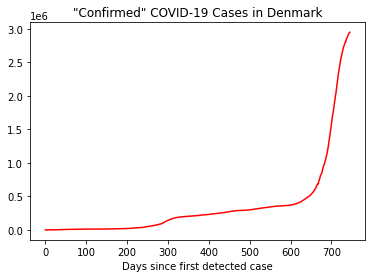
plt.plot(x,y, linestyle='-', color='r')
plt.title('"Confirmed" COVID-19 Cases in Denmark')
plt.xlabel('Days since first detected case')
Text(0.5, 0, 'Days since first detected case')
N = 5792202 # estimated population of DK in 2020
i_0 = y[0]/N # initial prevalence
x = np.array(range(len(y)))
# fit the model by nonlinear least squares
popt, pvoc = curve_fit(f, x, y, p0=[1, 0.5], bounds = (0, [500, 1]), maxfev=10000)
popt
array([2.11506788e-02, 4.12605498e-16])
S, I, R, C = sir_model(N, i_0, beta=popt[0], gamma=popt[1], delta=0, steps=len(y))
times = list(range(len(y)))
fig, ax = plt.subplots(nrows=1, ncols=1)
ax.plot(times, y, linestyle='-', color='r', label='Data')
ax.plot(times, C, linestyle='-.', color='k', label='SIR Model')
ax.legend(loc='best')
plt.xlabel('Days since first detected case')
plt.title('"Confirmed" COVID-19 Infections in Denmark')
plt.show()
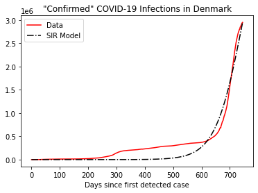
What happens if we run the model into the future?
S, I, R, C = plot_sir(N, i_0, beta=popt[0], gamma=popt[1], delta=0, steps=1000, verbose=True)
The total number of infections stabilizes, and the pandemic abates. The effective reproductive number \(R_0\) is less than 1.
Let’s do a quick sanity check. Recall that \(R_0 = \beta/\gamma\) for the SIR model initially, when the number infected, recovered, or dead are negligible compared to the total population. Once some of the population has recovered, some of the people an infectious person encounters wiil be people who have recovered and not susceptible to reinfection (according to the model). To first order, \(\beta\) is effectively reduced by \(S/N\).
# R_0 at the time the first infection is detected
popt[0]/popt[1] # greater than 1. According to the model, the infection will spread if R_0 > 1.
51261262636618.664
# After 1000 timesteps, R_0 is different
(S[-1]/N)*popt[0]/popt[1] # less than 1: According to the model, the infection will abate.
219047240451.27252
Fitting curves to the cumulative incidence function
The SIR model and its variants attempt to capture the dynamics of transmission and recovery, For some parameter choices, that leads to a sigmoidal shape for the cumulative incidence of infections.
Some pandemic predictions simply fit a sigmoidal function to the cumulative number of infections, an approach that dates back to William Farr in the 1800s. King et al. (2015) showed that this approach does not work well for AIDS or Ebola. Nonetheless, this is the approach the IHME takes: they fit a scaled and shifted Gaussian cdf to cumulative incidence.
Sigmoidal Models
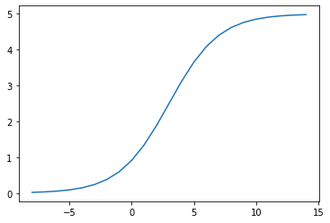
Common sigmoidal models include CDFs of unimodal distributions (such as the Gaussian cdf \(\Phi(x)\)) and the sigmoid function \(1/(e^{-x} + 1)\), the inverse of the logistic function.
To allow this function to be shifted and scaled, we can introduce the family of curves
The parameter \(a\) controls where the function crosses \(c/2\); \(b\) controls how rapidly it increases, and \(c\) is its asymptotic limit.
Let’s fit this to the Danish data.
def g(x, a, b, c):
    '''
    Wrapper for the sigmoid to pass to the curve-fitting function
    '''
    return c/(np.exp(-b*(x-a))+1)
# test g visually.
z = np.array(range(-8,15,1))
plt.plot(z, g(z,3,1/2,5))
[<matplotlib.lines.Line2D at 0x7f98b0dde0a0>]
# fit the DK data
popts, pvocs = curve_fit(g, x, y, p0=[len(x)/2, 0.02, np.max(y)/2], bounds = ([0, 0, 0], [500, 500, N]), maxfev=10000)
popts
array([5.00000000e+02, 1.11921669e-02, 1.16292975e+06])
# plot
Cs = g(x, popts[0], popts[1], popts[2])
times = list(range(len(y)))
fig, ax = plt.subplots(nrows=1, ncols=1)
ax.plot(times, y, linestyle='-', color='r', label='Data')
ax.plot(times, C[:len(times)], linestyle='-.', color='k', label='SIR Model')
ax.plot(times, Cs, linestyle=':', color='b', label='Sigmoid Model')
ax.legend(loc='best')
plt.xlabel('Days since first detected case')
plt.title('"Confirmed" COVID-19 Infections in Denmark')
plt.show()
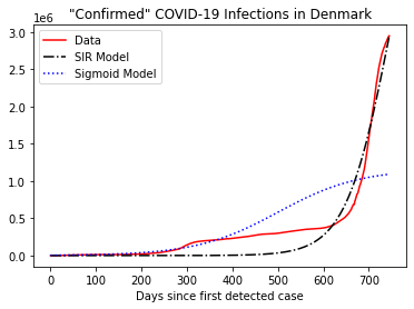
Both models agree reasonably well with past data. But they have rather different predictions about the future.
Let’s look at how the predictions vary over time, as the dataset grows.
def plot_predictions(y, n, points):
    '''
    plot SIR and sigmoid models fitted to the first n data

    Parameters
    ----------
    y : list of floats
        number of infections at each time point
    n : int
        fit the models to the first n elements of y
    points : int
        number of time points for which to plot the prediction

    Returns
    -------
    no return value
    '''
    # fit the two models
    x = list(range(len(y)))
    popt, pvoc = curve_fit(f, x[:n], y[:n], p0=[1, 0.5], bounds = (0, [500, 1]),
                           maxfev=10000)
    popts, pvocs = curve_fit(g, x[:n], y[:n], p0=[len(x)/2, 0.02, np.max(y)/2],
                             bounds = ([0, 0, 0], [500, 500, N]), maxfev=10000)
    times = list(range(points))
    S, I, R, C = sir_model(N, i_0, beta=popt[0], gamma=popt[1], delta=0, steps=points)
    Cs = g(times, popts[0], popts[1], popts[2])
    fig, ax = plt.subplots(nrows=1, ncols=1)
    ax.plot(x, y, linestyle='-', color='r', label='Data')
    ax.plot(times, C, linestyle='-.', color='k', label='SIR Model')
    ax.plot(times, Cs, linestyle=':', color='b', label='Sigmoid Model')
    ax.vlines(x[n-1], 0, np.max([C, Cs]), label='truncation time')
    ax.legend(loc='best')
    plt.xlabel('Days since first detected case')
    plt.title('"Confirmed" COVID-19 Infections in Denmark')
    plt.show()
interact(plot_predictions, y=fixed(y),
                           n = widgets.IntSlider(min=20, max=len(y), value=100),
                           points=fixed(2*len(y)))
<function __main__.plot_predictions(y, n, points)>
The predictions depend on the model and details of the data. A few additional days of data can drastically change the predictions. For some end dates, the two models have nearly identical predictions; for others, they differ by a factor of 20 or more.
Unlike the SIR model, the sigmoid model does not “know” how many people are in the population, so even if recovery conveys immunity, the cumulative number of infections in the sigmoid model can exceed the size of the population.
This mindless “curve fitting” approach is not a reliable basis for predicting the course of the pandemic, predicting ICU demand, predicting the effect of an intervention, allocating resources, or setting public policy. It is a mechanical application of models and algorithms to data, not science.
Unsurprisingly, models of this type do not predict infections well in practice. The most-cited predictions have been those promulgated by the Institute for Health Metrics and Evaluation (IHME) at the University of Washington. They say,
Our model is designed to be a planning tool for government officials who need to know how different policy decisions can radically alter the trajectory of COVID-19 for better or worse.
Our model aimed at helping hospital administrators and government officials understand when demand on health system resources will be greatest. (http://www.healthdata.org/covid/faqs#differences%20in%20modeling, last visited 23 January 2021)
IHME’s model is described here. Early in the pandemic, IHME predicted that there would be about 60,000 COVID-19 deaths in ths U.S. As of 18 February 2021, there have been more than 490,000. Between March and August, 2020, next-day deaths were within the IHME 95% prediction interval only about 30% of the time, despite revisions of the model https://arxiv.org/abs/2004.04734. (We shall not delve into how IHME produces its prediction intervals.) See also https://www.vox.com/future-perfect/2020/5/2/21241261/coronavirus-modeling-us-deaths-ihme-pandemic.
One feature of the sigmoidal models is that they predict rapid declines after the peak (the decline is just as rapid as the rise), a feature that some politicians like. That feature is built into the sigmoidal curve: it is an assumption, not something that comes from the data.
There are also more complicated models of pandemics, including models with more “compartments,” models based on other sigmoidal functions (such as the Gaussian CDF), and models that allow various kinds of heterogeneity within the population and simulate interactions between individuals. Some have proved more accurate than others. Just how poorly some models perform is obscured by the practice of revising the model and projections frequently–even daily.
Sometimes, a moddle with little substantive foundation can nonetheless predict the behavior of a system, at least if the system is not changing quickly. Accurate predictions of the effect of interventions (masks, lockdowns, vaccination, and so on) require a close tie between the world and the model: the model needs a substantive basis. For causal inferences, the model needs to be a generative model or response schedule.
George Box famously wrote, “all models are wrong, but some are useful.” While that quotation is often invoked as a general license to throw models at data, it should instead prompt questions:
useful for what?
how can you tell whether a model is useful for a particular goal?
In the same paper, Box wrote, “It is inappropriate to be concerned with mice when there are tigers abroad.” Most of the fretting people do about statistical models is at the level of mice (e.g., asymptotics under unrealistic assumptions), while the problems with most statistical models are tigers: the models have little or no connection to the actual scientific question.
New variants
As of this writing (10 February 2021), new strains of COVID-19 have been detected in the UK, South Africa, and the US, where cases of the new strain have a doubling time of about 10 days. The UK strain is estimated to be 50% to 70% more transmissible than the original virus. There is mounting evidence that the strain is also more lethal. https://www.wsj.com/articles/new-u-k-covid-19-variant-could-be-more-deadly-british-officials-say-11611338370 (last visited 22 January 2021).